A neural network is an essential aspect of Machine Learning. It can be easily understood as a system of computer hardware/software that works in a way inspired by mimicking the human brain. Through massive training, such a system learns from examples and generally without task-specific programming just like a real human does. In this article, I’m going to briefly explain the 27 neutral networks one by one in an easy-to-understand language.
1. Perceptron (P)
The simplest and oldest neural network we’ve known for a long time. It’s a linear classifier that takes in input, combines the input then maps to the corresponding outputs via particular functions. Nothing really fancy about it.
2. Feed Forward
Feed Forward is another oldest neural networks we know. It originated from the 1950s. A feed forward system generally includes the following:
- All nodes are linked
- No feedback loop to control the output
- There’s a layer between the input and output layer (the hidden layer)
In most cases, this type of network uses back-propagation methods for training.
3. Radial Basis Network
A radial Basis Network is actually a Feedforward with an activation function, a radial basis function instead of a logic function.
So what is the difference between these two kinds of networks?
A logic function maps an arbitrary value in the range [0, … 1] to answer the “yes or no” question. While this is applicable to a classification system it does not support continuous variables.
On the contrary, a radial basis function shows “how far we are from the target.” This is perfect for function approximation and machine control (For example, it can be a sub for PID controller).
In short, an RBF is an FF with different activation functions and applications.
4. Deep Feed Forward
DFF opened the Pandora’s Box for Deep Learning in the early 90s. These are still Feed Forward Neural Networks but with more hidden layers.
When training the traditional FF model, we only pass a small amount of error information to the next layer. With more layers, DFF is able to learn more about errors; however, it becomes impractical as the amount of training time required increases with more layers. Until the early 00s, we have developed a series of effective methods for training deep feedforward neural networks which have formed the core of modern machine learning systems today and enable the functionality of feedforward neural networks.
5. Recurrent Neural Network
RNNs introduce a different type of neuron: recurrent neurons.
The first network of this type is called the Jordan Network, where every hidden neuron receives its own output after a fixed delay (one or more iterations). Other than this, it is very similar to ordinary fuzzy neural networks.
Of course, there are other changes – such as passing state to the input node, variable delay, etc., but the main idea remains the same. This type of neural network is mainly used when the context is important – the past iterative results and the sample-generated decisions can impact the current ones. An example of the most common context is text analysis – a word can only be analyzed in the context of the preceding words or sentences.
6. Long/Short Term Memory(LSTM)
LSTM introduced a memory unit, a special unit that makes it possible to handle data along with variable time intervals. Recurrent neural networks can process text by “remembering” the first ten words, and LSTM long and short memory networks can handle video frames by “remembering” what happened from the many frames before. LSTM networks are also widely used for text and voice recognition.
The storage unit is actually made up of components called gates, which are recursive and control how the information is “remembered” and “forgotten”. The figure below illustrates the structure of LSTM:
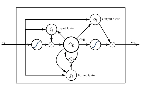
The above (x) is the gate, they have their own weight and sometimes have activation functions. On each sample, they decide whether to pass the data, erase the memory, and so on.
You can find a more comprehensive explanation of LSTM here:
http://colah.github.io/posts/2015-08-Understanding-LSTMs/
Inputting Gate determines how much of the last sample is stored in memory; the output gate adjusts the amount of data transferred to the next level, and the Forget Gate controls the rate at which memory is stored.
7. Gated Recurrent Unit
GRU is an LSTM with different gates.
The lack of an output gate makes it easier to repeat the same output multiple times based on a specific input. It is now most often used in sound (music) and speech synthesis.
Though the actual combination is a bit different: all LSTM gates are grouped together into a so-called Update Gate and the Reset Gate is closely related to the input.
They consume fewer resources than LSTM but have almost the same effect.
8. Auto Encoder
Autoencoders are used for classification, clustering, and feature compression.
When you train a feed forward (FF) neural network for classification, you mainly have to provide X examples in Y categories and expect one of the Y output cells to be activated. This is called “supervised learning.”
On the other hand, auto-encoders can be trained without supervision. Their structure – when the number of hidden units is less than the number of input units (and the number of output units equals the number of input units), and automatic encoder is trained in a way that the output as close to the input as possible, the automatic encoder is forced to generalize the data and search for common features.
9. Variational Auto Encoder
Compared with an autoencoder, a VAE compresses the probability, not the feature.
In spite of this simple change, an autoencoder can only answer questions like, “How do we summarize the data?”, while a VAE answers questions like “How strong is the connection between the two things? Should we divide the error between two things or are they completely independent? “
The more in-depth explanation can be found here: https://github.com/kvfrans/variational-autoencoder
10. Denoising Auto Encoder
Although auto-encoders are cool, they sometimes fail to find the most proper features but rather adapt to the input data (in fact an example of over-fitting).
The Noise Reduction Automatic Encoder (DAE) adds some noise to the input unit – changing data by random bits, randomly shifting bits in the input, and so on. By doing this, a forced noise reduction auto-encoder reconstructs the output from a somewhat noisy input, making it more generic, and forcing the selection of more common features.
11. Sparse Auto Encoder
Sparse Auto Encoder (SAE) is another form of auto encoding that sometimes pulls out some hidden packet samples from the data. The structure is the same as AE, but the number of hidden cells is greater than the number of input or output cells.
12. Markov Chain
Markov Chain (MC) is an old chart concept. Each of its endpoints is assigned a certain possibility. In the past, we have used it to construct a text structure like “dear” appears after “Hello” with a probability of 0.0053%, and “you” appears after “hello” with a probability of 0.03551%.
These Markov chains are not typical neural networks. They can be used as probability-based categories (like Bayesian filtering), for clustering (for some categories), and also as finite state machines.
13. Hopfield Network
The Hopfield Network (HN) is trained by a limited set of samples so that they react to known samples using the same sample.
Before training, each sample is used as an input sample, as a hidden sample during training, and as an output sample after it has been used.
When HN tries to reconstruct the trained samples, they can be used to denoise the input value and repair the input. If half of the pictures or sequences are given for learning, they can feed back to the entire sample.
14. Boltzmann Machine
Boltzmann machine (BM) is very similar to HN, with some cells marked as inputs as well as hidden cells. When the hidden unit updates its status, the input unit becomes the output unit (In training, BM and HN update units one by one instead of in parallel).
This is the first network topology that successfully preserves the simulated annealing approach.
Multi-layered Porzman machines can be used for so-called deep belief networks (to be introduced shortly), and deep belief networks can be used for feature detection and extraction.
15. Restricted Boltzmann Machine
The restricted Boltzmann machines (RBMs) are very similar to BMs in structure, but constrained RBMs are allowed to be trained back-propagating like FFs (the only difference is that the RBM will go through the input layer once before data is backpropagated).
16. Deep Belief Network
Deep Belief Network (DBN) is actually a number of Boltzmann machines (surrounded by VAE) together. They can be linked together (when one neural network is training another), and data can be generated using patterns learned.
17. Deep Convolutional Network
Today, Deep Convolutional Network (DCN) is the superstar of artificial neural networks. It has convolutional units (or pools) and kernels, each for a different purpose.
Convolution kernels are actually used to process incoming data, and pooling layers are used to simplify them (in most cases using nonlinear equations such as max) to reduce unnecessary features.
They are usually used for image recognition, they run on a small part of the image (about 20×20 pixels). The input window slides one pixel by pixel along the image. The data then flows to the convolution layer, which forms a funnel (compression of the identified features). In terms of image recognition, the first layer identifies the gradient, the second layer identifies the line, and the third layer identifies the shape, and so on, up to the level of a particular object. DFF is usually attached to the end of the convolution layer for future data processing.
18. Deconvolutional Network
The deconvolution network (DN) is the inverted version of DCN. DN can generate the vector as (dog: 0, lizard: 0, horse: 0, cat: 1) after capturing the cat’s picture. DNC can draw a cat after getting this vector.
19. Deep Convolutional Inverse Graphics Network
Deep Convolutional Inverse Graphics Network (DCIGN), looks like DCN and DN are attached together, but not exactly so.
In fact, it is an autoencoder, DCN and DN are not two separate networks, but rather a space that carries the network input and output. Most of these neural networks can be used in image processing and can process images that they have not been trained on before. For its level of abstraction, these networks can be used to remove something from a picture, redraw it, or replace a horse with a zebra-like the famous CycleGAN.
20. Generative Adversarial Network
The Generative Adversarial Network (GAN) represents the dual networks family consisting of generators and differentiators. They are always hurting each other – the generator tries to generate some data, and the differentiator receives the sample data and tries to discern which are the samples and which ones are generated. As long as you can maintain the balance between the training of the two neural networks, in the constant evolution, this neural network can generate the actual image.
21. Liquid State Machine
Liquid State Machines (LSMs) are sparse neural networks whose activation functions are replaced (not all connected) by thresholds. Only when the threshold is reached, the cell accumulates the value information from the successive samples and the output freed and again sets the internal copy to zero.
The idea comes from the human brain, these neural networks are widely used in computer vision, and speech recognition systems, but have no major breakthrough.
22. Extreme Learning Machine
Extreme Learning Machines (ELM) reduce the complexity behind an FF network by creating a sparse, random connection of hidden layers. They require less computing power, and the actual efficiency depends very much on tasks and data.
23. Echo State Network
An echo status network (ESN) is a subdivision of a repeating network. Data passes through the input, and if multiple iterations are monitored, only the weight between hidden layers is updated after that.
To be honest, besides multiple theoretical benchmarks, I don’t know any practical use of this Network. Any comments is welcomed.
24. Deep Residual Network
Deep Residual Network(DRN) passes parts of input values to the next level. This feature makes it possible to reach many layers (up to 300 layers), but they are actually recurrent neural network(RNN) without a clear delay.
25. Kohonen Network
Kohonen network (KN) introduces the “cell distance” feature. For the most part, used for classification, this network tries to adjust its cells to make the most probable response to a particular input. When some cells are updated, the cells closest to them are also updated.
Much like SVM, these networks are not always considered “real” neural networks.
26. Support Vector Machine
Support Vector Machines (SVMs) are used for binary categorical work and the result will be “yes” or “no” regardless of how many dimensions or inputs the network processes.
SVMs are not always known as neural networks.
27. Neural Turing Machine
Neural networks are like black boxes – we can train them, get results, and enhance them, but most of the actual decision paths are not visible to us.
The Neurological Turing Machine (NTM) is trying to solve this problem – it is an FF after extracting memory cells. Some authors also say that it is an abstract version of LSTM.
Memory is content-based; this network can read memory based on the status quo, write memory, and also represents the Turing complete neural network.
I hope this summary will be helpful to anyone that’s interested in learning about Neural Networks. If you feel like anything needs to be corrected or added, please contact us at support@octoparse.com.