Excel is one of the must-have data analysis tools in the market. To this day it provides more than 450 functions, but knowing how to use a few of them would be sufficient in most cases. In this article, I compiled 10 easy but widely used functions to facilitate data analysis in Excel. Feel free to try them out!
Sort & Filter
When dealing with a large amount of data, people may get confused and don’t know where to start. Sorting the information first will make it clearer to you. Excel allows you to sort data in ascending descending, and alphabetical order, etc.
For example, I extracted some business information from Yellowpages.com. In this spreadsheet, you can see the names of the stores, addresses, phone numbers, open hours, etc. Let’s say we want to rearrange the stores according to their names. Select the first row and choose “Sort & Filter” under the “editing” group, and then you can select the order you want your data to be sorted.
LEFT/RIGHT
Many people may not know that Excel allows you to extract the “X” number of characters from the beginning/end of cells. Staying with the Yellowpages example, to break down the phone numbers of businesses, =LEFT(Select cell, 3) can help extract the area code from phone numbers and =RIGHT(Select cell, 4) can get the last 4 digits.
Conditional formatting
Conditional formatting is useful when you want to sort out certain data that is valuable to you, especially when it comes to numbers. Let’s say I want to find out all the flatshare & houseshare in Australia that are under $200. I can first scrape the housing information from Gumtree.com, and then select “conditional formatting” under the “styles” group. There are many formatting options to choose from according to your needs. In this case, we can choose “greater than” and set up criteria for $200, and highlight them in yellow.
Remove Duplicates
It is common to have duplicated values in your spreadsheet. To remove the duplicated info, you can first highlight the duplicated data using the “conditional formatting” function (Optional, this will make sure the duplicates are obvious enough to locate so that we won’t miss any)
Then, use the “remove duplicates” function on the Data tab in the Data Tools section. Make sure you only select the column that contains duplicated values rather than the entire sheet.
TRIM
Sometimes you may find unwanted spaces in your cells, and it would be a huge waste of time to manually delete them. For instance, if the text you have in hand is full of spaces, just like the tweets I extracted from Twitter below (which is usually not the case), you can trim off the excessive part with an easy =TRIM(text) formula.
LEN
It is pretty easy to count words & characters in word documents and google docs, but what about in Excel sheets? LEN is a formula that helps you count the number of characters in cells automatically. When I was trying to determine the correlation between the lengths of YouTube video titles and their popularity, I scraped YouTube channel video information and used =LEN(text) formula to count the characters within a minute.
VLOOKUP
As one of the most frequently used functions, vlookup is popular to search for data associated with a value you enter. To explain how to use it, let’s first take a look at its formula:
=VLOOKUP(lookup_value, table_array,col_index_num, [range_lookup])
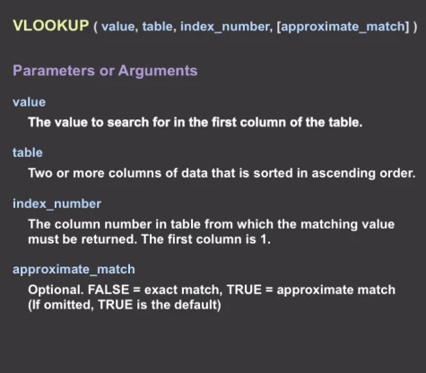
I know what you are thinking: what is this? It may seem a little confusing at first sight, but once you get the hang of it, it is really easy.
This time, let me take the cryptocurrency market data I got from Yahoo Finance as an example. Vlookup can search for the first column and find the matching value in the second column. Let’s say we want to find the symbol of cryptocurrency matching price 0.0013. First, sort out the info in ascending order. Next, select the two columns. Third, enter number “2” since we are trying to fetch data from the second column. Finally, choose FALSE to ensure an exact match of data. As you can see in the gif below, the corresponding value “ATB-USD” is returned.
COUNTIFS
This is another simple but useful Excel formula that is widely used. If it is not feasible to count the cells one by one to find out how many of them meet your criteria, you may consider taking advantage of this formula:
=COUNTIFS(criteria_range1, criteria1, criteria_range2, criteria2)
To understand it fully, imagine you are trying to figure out the number of male and female employees in each department of your company. To slice out the data with the COUNTIFS formula, you may select the data range and criteria. The first criteria range is the departments they are in, the second is their gender. In the example shown, the formula would be
=COUNTIFS(F11: F21, F13, G11: G21, G13)
Pivot table
The pivot table gives most people headaches. We all have heard how powerful it is but only a few can use it well. A Pivot table allows you to quickly summarize and analyze large amounts of data in lists and tables by dragging and dropping columns to different rows or columns. The columns can also be re-arranged as you wish.
SUMPRODUCT
When you have a number of items with their quantities and prices in hand and you want to figure out their total sales, you may take advantage of this function. SUMPRODUCT multiplies the quantity of each item and its price, and then adds up the sales of each item to deliver the total sales.